For many years I served on an AICPA committee to develop standards for CPAs to follow when design spreadsheets. The goal was help CPAs create spreadsheets with consistent designs so that they could be more easily used and reviewed by one another. This somewhat dated, but interesting information is presented below.

Design Standards for Financial Planning Spreadsheets
1. Separate your assumptions from your formulas.
2. Minimum documentation.
3. Use cross-footing formulas to prevent and detect errors.
4. Complex formulas should be broken in to several formula.
Power Tools for Financial Planning
1. Using Data Tables for What-If Analysis.
2. Using Lookup Tables for Tax Rate Schedules.
3. Considering Alternatives with Backsolver & Version Manager.
4. Using Graphics for Analysis and Presentation of Results.
Add Power to Your Results by Dressing Up Your Report
Effective Budgeting and Forecasting
Prepared and Presented by:
Will B. Rich, CPA, PhD
Design Standards for Financial Planning Spreadsheets
Quality control is a necessary element of all information systems that provide accurate information. Electronic spreadsheets are extremely flexible and very unstructured. While these attributes are part of the beauty of electronic spreadsheets they significantly increase the risk of errors. Unlike very structured financial software (ex. tax processing software) users can modify formula and assumptions without realizing that these modifications may result in unintended results in other areas of the spreadsheet.
There are numerous examples of CPA firms and accounts in industry making errors in constructing electronic spreadsheets that have cost their organizations millions of dollars. For example, one large CPA firm made a mistake in helping a construction contractor prepare a bid on a high rise office building. Based on the spreadsheet calculations the contractor bid on the job, got the contract, and lost money. He successfully sued the CPA firm for $10,000,000.00. That's a lot of billable staff hours.
A few simple spreadsheet design standards can go a long way to reduce the risk of errors in spreadsheets. This conference paper does not attempt to provide a comprehensive list of spreadsheet standards. Rather only the key standards that should always be in place are included. The AICPA MAS Computer Applications Subcommittee is currently working of a Practice Aid that will contain a comprehensive list of electronic spreadsheet standards.
Quality control standards for electronic spreadsheets are not software specific and are important regardless of the software in use.
Separate Your Assumptions From Your Formulas
Many spreadsheets incorporate a number of assumptions (such as the rate of interest in a loan amortization table). The computation formulas should be made up completely of cell references; the assumptions should not be embedded in the formulas. For example, consider a Lotus 1-2-3® spreadsheet which uses the @PMT function to calculate a loan payment amount for a $50,000 loan with a 10% interest rate and a term of 15 years of monthly payments.
A poor way to write the formula would be: @PMT(50000,.1/12,15*12). A much better method places each of the four assumptions (i.e. the $50,000, the 10%, the 15 years and the 12 payments per year) in a separate cell (such as cells C6, C7, C8, and C9) and to write the formula as follows: @PMT(C6,C7/C9,C8*C9).
This method makes it easier and safer to change any of the assumptions (such as the interest rate). Furthermore, when the worksheet is printed, the printout will clearly reveal the assumptions used in the computation. If possible, assumptions should be placed in separate, clearly identified areas of the spreadsheet.
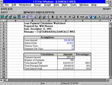
Figure 1. - Assumptions separated from formulas.
Include Minimum Documentation In All Spreadsheets.
a. Spreadsheet should be clearly titled.
b. Include "Prepared by: " on all spreadsheets.
c. Include drive, path, and filename on spreadsheet and in print area. An easy to do this is with the following formula:
@CELLPOINTER("FILENAME")
d. Include the date (and even the time if you are reprinting frequently) on each printout. A good way to do this is with a date formula. For example in Lotus 1-2-3 you could simply type in:
@TODAY of @NOW
If you don't want the date to change you can turn this formula into it's output with the {EDIT} {CALC} key sequence or with the Range Value command.
Use Cross-footing Formulas to Prevent and Detect Errors
Most accountants would not consider signing off on a manual worksheet that could be cross-footed without doing so. However, it is not uncommon for these same individuals to prepare electronic spreadsheets that could be cross-footed without doing so.
A simple way to cross-foot electronic worksheets is to build a formula with the @IF function. For example, assume you have a loan amortization schedule and the total for all payments is on cell B20, the total for all interest payments is on C20, and the total that was applied to principal is on D20 (see Figure 2. on the next page). You should place the following cross-footing formula somewhere on the worksheet:
@IF(B20=C20=D20,""."Error! Spreadsheet does not foot")
If the spreadsheet cross-foots, the cell appears empty (the "" stands for null string and makes the cell appear empty when the condition in the @IF function is true.)
If the spreadsheet does not cross-foot the Error message appears in the cell where the formulas is entered.
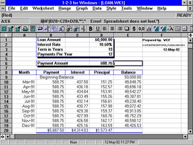
Figure 2. - Cross-footing formulas to prevent & detect errors.
Complex Formulas Should Be
Broken into Several Formulas
Long formulas are difficult to edit, understand, and review. A good rule of thumb is "if the entire formula can not be seen in the control panel, its' too long." Lookup tables can often be useful in shortening long complex formulas.
Power Tools for Financial Planning
Using Data Tables for What-If Analysis
Typically financial planning involves a great deal of what-if analysis. Electronic spreadsheets are ideal for what-if analysis because you can change one assumption and quickly find out how all of your calculations are affected. The major drawback of this type of what-if analysis is that when you change an assumption and the spreadsheet is recalculated, the old calculations disappear and are not available for comparison with the revised calculations.
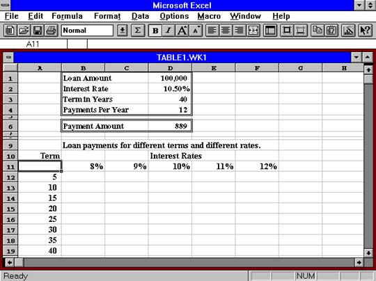
Figure 3. - What-If Analysis With Data Tables
Data tables solve this problem and also tremendously simplify very extensive what-if analysis (sometimes referred to as sensitivity analysis). They are easy to build, and generally easy to understand. Considering
that they are such a powerful and easy to use tool, it may seem odd that even advanced users rarely use them. Unfortunately, many spreadsheet users are not aware of data tables.
Using Lookup Tables for Tax Rate Schedules
Lookup tables allow the user to "lookup" information such as tax rates or brokerage commissions on a table rather than embedding the information in formulas. There are several important advantages of using lookup tables as opposed to creating long formulas.
Advantages of Lookup Tables:
1. With lookup tables there is no need to build long formula that are hard to understand and change, and have a high risk of errors.
2. Lookup tables allow the user to quickly and easily change the table information (ex. change the tax rates) without having to modify the formulas in the spreadsheet.
3. Lookup tables make it easy to see what assumptions the spreadsheet formulas are based on.
Lotus 1-2-3 provides for two types of lookup tables:
1. Vertical lookup tables @VLOOKUP in which the information is laid out in a vertical manner as is typical with tables such as tax rate schedules.
2. Horizontal lookup tables @HLOOKUP in which the information is laid out horizontally. Example: comparative income statements where the first row of the table is the year numbers.
Microsoft Excel also has Vertical and Horizontal lookup tables.
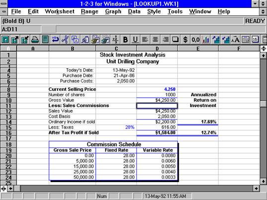
Figure 4. - Vertical Lookup Table
Considering Alternatives with
Backsolver & Version Manager
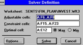
Lotus 1-2-3 provides a "Solver" and "Backsolver" utility that allows the user to optimize some specific objective (ex. net income from investments) based on certain constraints. In the following example the objective is to maximize after tax return on an investment portfolio.
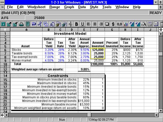
Figure 5. - Using Solver to Optimize Income
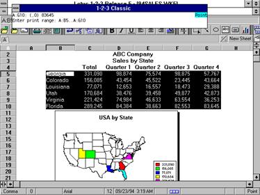
Using Graphics for Analysis & Presentation of Results
With electronic spreadsheets it is easy to accumulate massive amounts of detailed information for use in making financial decisions. For example, the spreadsheet on the next page provides a great deal of useful information for an individual who is considering refinancing a $100,000 long term loan at a lower interest rate. The key considerations in making such a decisions are the term of the loan and the resulting interest rate.
The graph at the bottom of this page does a much better job of communicating the "information" contained in the numbers than the chart on the next page does. As you can see from the graph, the size of the loan payment ceases to decrease materially for terms larger than 15 years. The graph also clearly illustrates that this conclusion is true for any of the interest rates within the relevant range.
Unfortunately, many accountants do little of no graphing in their financial presentations. With today's electronic spreadsheets, graphing it is easy to include top quality graphs with your financial presentations.
Add Power to Your Results by Dressing Up Your Report
Today's electronic spreadsheets make it easy to DTP (i.e. Desk Top Publish) your financial reports and projections. Features such as bold facing, shading, double underlines, graphs embedded in presentations, and much more are all both available and easy to learn and use. Surprisingly however, many accountants do not think its worth the time and effort. Examine the two short presentations below and you be the judge as to which looks the most professional.
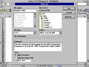
Save File Information
In Lotus 1-2-3 for Windows, the process of saving a file gives the user the opportunity to add addition text describing the file. This makes it easier to identify a file later for retrieval or deletion. In addition, this document information is accessible by LotusNotes for better group management of 1-2-3 files.
Lotus 1-2-3 looks at file structures, not extensions
Lotus 1-2-3 knows it’s files by their structure, not by their extension. You can name a 1-2-3 file anything you want, you just have to use the ESC key as outlined above to find the file you are looking for. In fact, the WK1 on 1-2-3 version 2.01 files was intended to be a version increment but not many people knew about this new undocumented feature. Many users on networks use their initials as the extension so they will only be looking at their files in large directories.
Using Backspace to cancel prior ranges
Lotus 1-2-3 has a habit of remembering prior ranges. Sometimes this is very helpful. More often this is a pain in the neck. Most 1-2-3 users will press the ESC key when a prior range appears, however this is not the best way to cancel prior ranges. Pressing the ESC key in many cases will still leave you at the prior range instead of where you were before the prior range popped up. Instead, try pressing the Backspace key. The Backspace key acts as a true range killer and will leave you exactly in the same place you were when the prior range popped up and took you for the magical, mystical ride to some prior range.
DEL key will delete ranges now.
You can use the delete or DEL key on a highlighted cell to erase the cell instead of using a range erase. The only disappointment is that this does not work on a range of cells, yet.
F4 WYSIWYG pre-highlight with the keyboard.
When you have WYSIWYG loaded you can pre-highlight a range to format, erase, and any other command by pressing the F4 key when in READY mode. This is especially useful when you want to execute a series of formatting commands from WYSIWYG.
UNDO - work with nets!
Lotus 1-2-3 version 2.2 and higher has an UNDO feature which allows you to undo your last goof. UNDO will take more memory when you have larger files as it has to be able to recover you from a complete worksheet erase command. Because of this, many users have turned the UNDO feature off when what they need to do is either buy more memory or optimize the memory they have better. Note, 1-2-3 versions 3+ do not have the memory problem that 2.X versions have due to a better memory scheme (Extended Memory, see below).
Using the Period key to examine ranges
Many times you may have a range that is too big to fit on the display and you want to examine the corners of the range. Lotus 1-2-3 allows you to switch the anchor of the range by pressing the period key. 1-2-3 always thinks that you have four corners even when all you have is two, like a column range. Give it a try, pressing the period key will move you from corner to corner without canceling the range. Just remember that when you want to move to the bottom of a column range it requires two periods not just one.
Top & Bottom line in @SUM functions, please
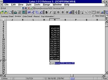
1-2-3 will not automatically adjust your @SUM functions when you insert lines or delete lines unless you have included a line above your first number and the line below your last number in a column of numbers. This is also important to note for those who are using the new AutoSum function. The newer versions of Lotus 1-2-3 and AutoSum will not add an additional line, but they will adjust properly for a line deleted at the beginning or end of a range.
F1 on @ and @ Functions
The context sensitive help in 1-2-3 is now helpful. Type @ and press F1, 1-2-3 opens up a help screen right to the entire list of the @ functions. Try it again by typing @PMT and press F1, this time 1-2-3 will open up the help screen right to the @PMT syntax screen and allow you to quickly review the syntax.
General format
Most 1-2-3 users will use the Fixed format when they have whole numbers under 1,000. This can be very hazardous if you mis-type a number and have pieces behind the decimal point that create problems with your formula. When this occurs the Fixed format will not show you your mis-type. General, on the other hand, will show you the exact number in the cell at all times based on the column width. The wider the column the more decimal places are displayed. Consider using General format for whole numbers under 1,000 to help you find typos quickly.
General can also be very helpful in finding a rounding problem in a section of the worksheet. Apply the General format, find the error, and reformat the data.
Mapping @IF functions
When it comes to @IF functions you can find yourself lost in the @IF zone in no time at all. To prevent you from becoming lost in the @IF zone, map out the logic in your conditional statements before you try to create the formula. This will help you make sure that the logic is correct before you start the formula, keep you from placing syntax in the wrong place, and help you make sure you have provided for all conditions possible. This is very important. In fact, many advanced users keep the logic map as part of the documentation for the worksheet to help with future revisions and prove logic if needed. A simple upside-down “Y” can do the trick quite nicely. See above graphic.
When using the upside-down “Y” certain sections can remind you of syntax. For example, anytime you see an intersection this could remind you that you need an “@IF(” in your formula. Also, when you go down a leg you cross of the leg and this can remind you to type a comma “,”in your formula and when you complete a leg you will know to place a solution in the formula. Last, when you have two completed legs it is time to remember to use the “)” right parenthesis to close that section. In summary:
· Intersection @IF(
· Leg , (comma)
· End of leg solution (dot solution)
· Two legs completed ) (close or right parenthesis)
If you use this method, it will also show you when you need to do the dreaded double parenthesis in the middle of a formula. Most users just guess on this one until they get it right. With this trick you can see it coming.
Zero suppression with “ “ in @IF functions
You can design your @IF functions to provide a zero suppressed look in all cases if you use “ “ (quote, space, quote) as an option in the function itself. Do not use the “” or (quote, quote) option as this will work but will read as a NULL cell to 1-2-3. A NULL cell is a completely blank cell and this could create problems with your macro, or function.
F4 the ABS key
Most users know that the F4 will add dollar signs to any formula when you are in point mode creating or editing a formula. However, they do not realize that the F4 is actually a four way toggle as follows:
1. add both dollar signs
2. remove one dollar sign
3. remove the other dollar sign , add the prior dollar sign back
4. remove all dollar signs
Note: Currently, all versions of 1-2-3 do not allow this on named range references only on non-named references.
Two precautions for sorting data
Before sorting data it is a good idea to save your file and also have a method to get to the original order in your worksheet. For example, if you are sorting a list of names and phone numbers, you may want to add a column and use data fill to give the data an original numbering sequence. This allows you to sort back easily without having to retrieve the saved file which sometimes may not be feasible if numerous changes have been made. It is always best to have both precautions to fall back on to protect your data.
Saving often
Save often. Saving should be a reflex for 1-2-3 users. Two rules come into play:
· Save before you do anything tricky
· Save the minute you have done anything at all you consider substantial
Do not play roulette with the power companies. It is a good idea to always save before printing, sorting, extracting, or combining worksheets.
Also, use the File Save Backup command before saving to the regular file name. This could prevent a disaster that may occur if the power goes off during the middle of the saving process.
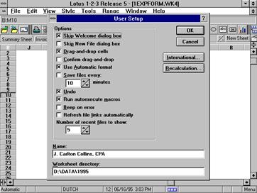
Lotus 1-2-3 for Windows has a new command which automatically saves your worksheet on a periodic basis. To use this feature, select Tools, User Set up, and click on the automatic save box shown below.
Save versions
Be sure to have different versions of your worksheet when you are working on an important project. The new version manager in 1-2-3 for Windows can help but the best way is to have separate files for each step of the development process. This way you can go back when you have created a mess. Remember, it is much harder to undo, than to do!
@Round, why, when & to what number of decimal places
Currently, there is no global rounding control in Lotus 1-2-3. Instead, you must round whenever your calculation returns pieces of your number. A good rule of thumb is as follows:
@ Round when you:
· Multiply
· Divide
· use an @ Function that returns numbers behind the decimal place
Even when you are multiplying whole numbers it is still best to round the multiplication in case you change your whole numbers in the future to have decimal places. In the future you will not remember that you did not round that particular calculation. Play it safe and round in all of the above three cases, if you do you can @SUM to your heart’s content and will never have a rounding error. (with the exception of the 1-2-3 negative zero bug)
Many 1-2-3 users will automatically round all their functions to two decimal places. This is and error. You should setup a rounding control cell and round to the number of decimal places in the cell. This way all your related @ROUND functions can reference this one cell for rounding control. This is as close to global rounding control as you can come with 1-2-3.
@ROUND control decimals
|
-3 nearest -1,000 |
1 nearest 10 |
|
-2 nearest -100 |
2 nearest 100 |
|
-1 nearest -10 |
3 nearest 1,000 |
|
0 0 or whole numbers |
|
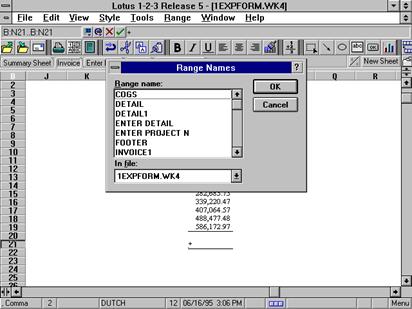
F3 in formula creation for Range Names
Use the F3 key to pop-up range names when you are creating formulas. This allows you to simply highlight the range name you want to use in the formula and viola 1-2-3 does the typing for you.
Copy every other cell, or so
By inverting the from (what) and to(where) ranges in the copy command you can easily copy data to every other cell, every third cell, every fourth cell, and so on.

Step one issue the copy command and elongate the what or from range.

Step two, point at a single cell for the where or to range down the exact number of cells you want to skip each time. Hit the enter key and...

Viola, you have done the every other or so copy. If you watch the ranges carefully you can pick up on the logic that makes this trick work.
Watch out for errant text or typos in Macros
Macros can be like charging freight trains. The only way a macro will stop is if it encounters a blank cell or a quit command. Watch out for text that slips into the path of the macro as you may get more than you bargain for.
Simple Grand Total
Quite frequently users will setup a worksheet with detail and subtotals and have problems with a grand total that is the total of the subtotals. The problem comes when they want to add or delete sections. The trick is to subtotal all data and then at the bottom merely total everything and divide by two.
Another method is to use the new @Subtotal and @GrandTotal functions included in Lotus 1-2-3 5.0 for Windows.
Case Studies
Using Oldies But Goodies Hints & Tips
Use Data Tables for What-If Analysis.
Typically financial planning involves a great deal of what-if analysis. Electronic spreadsheets are ideal for what-if analysis because you can change one assumption and quickly find out how all of your calculations are affected. The major drawback of this type of what-if analysis is that when you change an assumption and the spreadsheet is recalculated, the old calculations disappear and are not available for comparison with the revised calculations.
Data tables solve this problem and also tremendously simplify very extensive what-if analysis (sometimes referred to as sensitivity analysis). They are easy to build, and generally easy to understand. Considering that they are such a powerful and easy to use tool, it may seem odd that even advanced users rarely use them. Unfortunately, many spreadsheet users are not aware of data tables.

Lookup Tables
Lookup tables allow the user to "lookup" information such as tax rates or brokerage commissions on a table rather than embedding the information in formulas. There are several important advantages of using lookup tables as opposed to creating long formulas.
Advantages of Lookup Tables:
a. With lookup tables there is no need to build long formulas that are hard to understand and change, and have a high risk of errors.
b. Lookup tables allow the user to quickly and easily change the table information (ex. change the tax rates) without having to modify the formulas in the spreadsheet.
c. Lookup tables make it easy to see what assumptions the spreadsheet formulas are based on.
|
|

Lotus 1-2-3 provides for two types of lookup tables. Vertical lookup tables @VLOOKUP in which the information is laid out in a vertical manner as is typical with tables such as tax rate schedules. Horizontal lookup tables @HLOOKUP in which the information is laid out horizontally. Example: comparative income statements where the first row of the table is the year numbers.
Solver and Backsolver
Lotus 1-2-3 provides a "Solver" and "Backsolver" utility that allows the user to optimize some specific objective (ex. net income from investments) based on certain constraints. In the DOS version of 1-2-3, Solver and Backsolver are Add-ins that ship with the 1-2-3 code. In the Windows version of 1-2-3, there are menu choices. In the following example the objective is to maximize after tax return on an investment portfolio.


Solver dialog box from Lotus 1-2-3 for Windows Release 5.0
Using Graphics
With electronic spreadsheets it is easy to accumulate massive amounts of detailed information for use in making financial decisions. For example, the spreadsheet on the next page provides a great deal of useful information for an individual who is considering refinancing a $100,000 long term loan at a lower interest rate. The key considerations in making such a decisions are the term of the loan and the resulting interest rate.
|
|

The graph at the bottom of this page does a much better job of communicating the "information" contained in the numbers than the chart on the next page does. As you can see from the graph, the size of the loan payment ceases to decrease materially for terms larger than 15 years. The graph also clearly illustrates that this conclusion is true for any of the interest rates within the relevant range.

Graphics in 1-2-3 are not limited to traditional graphs. All versions now ship with "clip-art" images that can be easily added to the worksheet. Use the : Graph Add Metafile command to import these images.

One of the subtle but significant improvements to 1-2-3 has been the ability to include "live" graphs in worksheets. Live graphs first came to 1-2-3 with Release 2.3 and WYSIWYG. These "live" graphs can be placed on the face of the worksheet and change as the numbers change.

@CELLPOINTER("filename")
The @CELLPOINTER function can be used to calculate various "attributes" for the cell that currently contains the pointer. Those attributes include the address, column, contents, format, prefix, protection status, row, type of data in the cell (i.e. blank, value or label, width, or the path and filename of the active file. The function is typed as follows:
@CELLPOINTER("filename")
If you type in this function and you have not yet named the file, the cell will appear to be blank. If you are going to change the filename or save the file to a different location, do so before you print so that the new path and filename will appear on the printout. You will have to press the {CALC} key to have the worksheet recalculated after you save the file with a new name.
If you wish to have the path and filename information included in a header or footer you can use the backslash (i.e. \) and the cell reference containing the @CELLPOINTER formula when 1-2-3 prompts you for the header or footer information. For example, if the @cellpointer("filename") function is in cell d3 you would put \d3 where the prompt is asking for the header or footer.
Use the Data Fill Command to Fill in Dates.
|
|

The Data Fill command enters a sequence of values in a specified range. You can enter a sequence of numbers, dates, times, or percentages. To fill a range with sequential dates you use special start, step, and stop values.
To fill a range with dates, enter the start value as a date in any one of the 1-2-3 date formats except short international. For example, you could enter 3/27/91 as the start value. 1-2-3 makes some assumptions about the date you enter when you use certain formats. For example, if you enter May-91, as the start value, 1-2-3 will assume you mean Ol-May-91. If you enter 27-May without a year, 1-2-3 will assume you mean to use the current year.
When entering the step you may use the following letter:
d for day,
w for week,
m for month,
q for quarter, or
y for year.
, for eternity as in “postal mail service”.
These letters must be proceeded by an integer. For example, using 1m as the step would mean that the step was 1 month. Using 4w as the step would mean that the step was 4 weeks.
String Arithmetic
String arithmetic is the ability to add labels together. It is a simple operation and works in all versions of 1-2-3 from 2.0 up. You simply use the ampersand (i.e. the &) as the operator rather than the +.

String Arithmetic and the string @ functions (i.e. @CLEAN, @FIND, @LEFT, @RIGHT, @LENGTH, @PROPER, @TRIM, etc.) can also be useful for converting database and other ASCII information to columnar format.
Use String Arithmetic to Clarify Line Items in Budgets
Budgets and other financial presentations, such as the one provided below can often be enhanced by modifying the labels to disclose additional information.

Contents of Cell A20 before the unit information is added:
‘Sales Revenue
The following is an example of how string arithmetic can be used to modify some of the labels to disclose this additional information:

Contents of Cell A20 after the unit information is added:
+"Sales Revenue "&"("&@STRING(D20/D17,0)&" units)"

Use Circular References to
Solve Simultaneous Equations
Some worksheets will necessarily involve circular references. For example, in computing accrued state taxes you may need to know federal tax expense. However, to compute federal taxes you may need to know state tax expense. You simply construct the formula as logic would dictate and then turn on / Worksheet Global Recalculation Iterations to a large enough number until the correct solution is reached the first time an input number is changed.

|
|

|
|

Use cross-footing formulas to prevent and detect errors
Most accountants would not consider signing off on a manual worksheet that could be cross-footed without doing so. However, it is not uncommon for these same individuals to prepare electronic spreadsheets that could be cross-footed without doing so.
A simple way to cross-foot electronic worksheets is to build a formula with the @IF function. For example, assume you have a loan amortization schedule and the total for all payments is on cell B20, the total for all interest payments is on C20, and the total that was applied to principal is on D20 (see Figure 2. on the next page). You should place the following cross-footing formula somewhere on the worksheet:
@IF(B20=C20=D20,""."Error! Spreadsheet does not foot")
If the spreadsheet cross-foots, the cell appears empty (the "" stands for null string and makes the cell appear empty when the condition in the @IF function is true.)
If the spreadsheet does not cross-foot the Error message appears in the cell where the formulas is entered.

Passwords & / File Admin Seal
You can password protect your files by pressing the spacebar and typing the letter P after you type in a file's name during file save. This works in all versions of 1-2-3. However, as is frequently the case with passwords, if you forget your password you are in trouble. It is almost impossible to open a password protected file without the password. There is, however, at least one third party software package that will break passwords, so they are not completely secure. Further, the password does not affect the file attributes of a file and therefore will not prevent someone form erasing the file from the disk.
You can prevent others from turning off Global Protection with the File Administration Seal command. To seal a file you must assign a password (this is a different password than the one you may choose to assign to prevent others from retrieving your file). The seal can not be disabled without knowing the password. When you seal a file, the following commands are sealed and cannot be used to change the file:
/ File Admin Reservation Setting
/ Graph Name [Create, Delete, Reset]
/ Print [E,F,P] Options Name [Create, Delete, Reset]
/ Range Format, Label, Name, Prot, Unprot
/ Worksheet Column, Hide, Global
Use A Simple Macro to Enter A Column of Numbers
The simplest way to enter a column of numbers is to create a simple macro such as the following:
\t {?}/100{CALC}{D}{BRANCH \t}
Since this is a temporary macro I would follow my customary naming convention of naming the macro \t.
Specify Multiple Print Ranges
You can specify multiple print ranges simultaneously by separating the different ranges with a comma. For example, a valid print range would be a1..e32, a50..392. This will not work in release 2.x and will not work with the old / Print Printer Range command in Release 3.x and 1-2-3 for Windows.
Double Label Prefix Symbols

To have a label centered around a cell (example in cell b3 ) you proceed the label with ^ ^. To have the label right aligned you use " " as the label prefix symbol. The Range Justify and :Text commands are also useful in dealing with sentences and paragraphs.
/ Range Format Other Command
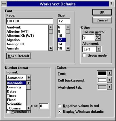
The easiest way to format the cell in advance of data entry is to use the Automatic Format setting under the Style, Worksheet defaults, menu item.

The automatic format is particularly useful when you are entering in a variety of numbers that have different formats. With the automatic format, 1-2-3 will automatically format the cell based on what you type in. For example, if you enter $3,456.98 then 1-2-3 will enter the number 3456.98 in the cell and format the cell in the currency format with 2 decimal points. The following are some examples of the output of the Range Format Other Automatic command:
You Enter 1-2-3 Displays Cell Contents
3,234.56 3,234.56 (,2) 3234.56
$567.92 $567.92 (C2) 567.92
125 Oak Street 125 Oak Street (L) '125 Oak Street
@sum(a:al.. @sum(a:al.. (L) '@sum(a:al..
27-Mar-92 27-Mar-92 (Dl) 33690
32.8% 32.8% (PI).328
| (Pipe) Symbol For Sophisticated Data Query
Assume you are managing the following database using 1-2-3 and periodically you print a report of inventory on hand. However, you wish to print one report for the Monroe warehouse and one report for the Lafayette warehouse.
|
|

Notice the formula in cell I24 . It uses the @IF to place the | (pipe symbol also called the split vertical bar) in column A for all records where the location is not equal to the contents of cell H19.
As you may recall if you're a long time 1-2-3 user, placing the pipe symbol as the first character in the first column of any row in a print range causes that row not to print. In the days before WYSIWYG we used to use this symbol to embed print setup strings in documents or to create remark lines that were not printed. If the worksheet is printed without changing the cell H19, the following will be the result:

Macro Menus
Most advanced users have numerous macros in the worksheets they use frequently. It is often a time consuming task to locate the macros, find out what they do and determine their names. In a worksheet where there are a number of macros the MENUCALL and MENUBRANCH macro commands can be used to streamline and simplify the process of using the macros. In 1-2-3 for Windows you can also use the MENUCREATE and MENUINSERT commands.
Assume, for example, you have four macros in a worksheet named \p, \s, \t, and \q. The \e macro automates data entry, the \p macro prints a report, the \s runs a macro that uses the GETNUMBER command to prompt the user for a number that will be placed in a cell named price, \t uses the GETNUMBER command to prompt the user for a number that will be placed in a cell named rate, and the \q informs the users that he can not get out of this macro.
All of these macros could be automated by building a macro front end as follows: